Talent vs Luck: A Critical Response

The ‘Talent vs Luck’ simulation paper’s conclusion that luck dominates talent is baked into the model from the start — here’s the math showing why.

The paper “Talent vs Luck: the role of randomness in success and failure” (journal, arXiv) by Pluchino, Biondo, and Rapisarda was covered in MIT Technology Review and Scientific American, and later won the 2022 Ig Nobel Prize in Economics. The authors build a simulation — the Talent vs Luck model (TvL) — and conclude:

We can conclude that, if there is not an exceptional talent behind the enormous success of some people, another factor is probably at work. Our simulation clearly shows that such a factor is just pure luck. — Pluchino, Biondo, Rapisarda

We argue this conclusion is baked into the structure of the model from the start.

In the TvL model a person in the 95th percentile of talent has roughly a 6.1% chance of doubling their capital each timestep; a person in the 5th percentile has 3.4%. The difference between extreme outliers is only ~2.6 percentage points per timestep. Starting from such a small difference between talent levels essentially guarantees the conclusion before the simulation even runs.

What makes the model’s outcome inevitable is its multiplicative structure. While the average capital grows slightly for talented people, the geometric-mean growth rate — which governs typical long-run paths — is negative for everyone with talent below 1. A few lucky individuals capture enormous gains, pulling the arithmetic mean up, while for realistic talent levels in this model, most people lose capital. This asymmetry is baked into the model by construction: talent can help you capitalize on lucky events, but it offers zero protection against unlucky ones.

The TvL Model

A high-level description of the model from the paper:

• \(N\) people are placed uniformly at random in a square environment and stay fixed.
• \(N\) events are also placed uniformly at random, each classified as Lucky or Unlucky (50/50).
• The events randomly walk the environment each timestep.
• At each timestep, capital is updated:
  • No overlap with an event: capital unchanged.
  • Overlap with an Unlucky event: capital halved.
  • Overlap with a Lucky event: if a uniform random draw \(u \in [0,1)\) is less than the person’s talent score, capital doubles; otherwise unchanged.

Talent is drawn from \(\mathcal{N}(0.6,\ 0.1^2)\), truncated to \([0,1]\). Everyone starts with 10 units of capital and the simulation runs for 80 timesteps.

The one parameter the paper does not give explicitly is \(p_\text{event}\) — the probability that a given person overlaps an event at a given timestep. We estimate it in the appendix; our best estimate is 0.16.

Setup

import numpy as np
import matplotlib.pyplot as plt
import scipy.stats as ss

rng = np.random.default_rng(seed=20180312)

# Paper's parameters
N_PEOPLE = 1000
N_TIMESTEPS = 80
STARTING_CAPITAL = 10.0
TALENT_MEAN = 0.6
TALENT_SD = 0.1
P_LUCKY = 0.5

# Our estimate of p_event (derived in appendix)
P_EVENT = 0.16

Simulating the TvL model

def run_tvl_simulation(n_people=N_PEOPLE, n_timesteps=N_TIMESTEPS,
                       starting_capital=STARTING_CAPITAL,
                       talent_mean=TALENT_MEAN, talent_sd=TALENT_SD,
                       p_event=P_EVENT, p_lucky=P_LUCKY, rng=rng):
    """Run the TvL simulation; returns (talent array, final_capital array)."""
    talent = np.clip(rng.normal(talent_mean, talent_sd, n_people), 0, 1)

    # Pre-draw all random numbers: shape (n_people, n_timesteps)
    event_roll   = rng.random((n_people, n_timesteps))
    lucky_roll   = rng.random((n_people, n_timesteps))
    capital_roll = rng.random((n_people, n_timesteps))

    event_happens = event_roll < p_event
    is_lucky      = lucky_roll < p_lucky
    capitalizes   = capital_roll < talent[:, np.newaxis]

    # multiplier per (person, timestep)
    multiplier = np.where(
        event_happens & is_lucky & capitalizes, 2.0,
        np.where(event_happens & ~is_lucky, 0.5, 1.0)
    )

    final_capital = starting_capital * multiplier.prod(axis=1)
    return talent, final_capital

talent, final_capital = run_tvl_simulation()
print(f"Median final capital:  {np.median(final_capital):.3f}")
print(f"Mean final capital:    {np.mean(final_capital):.3f}")
print(f"Max final capital:     {np.max(final_capital):.1f}")
print(f"Fraction who grew:     {(final_capital > STARTING_CAPITAL).mean():.1%}")

Median final capital:  1.250
Mean final capital:    26.164
Max final capital:     5120.0
Fraction who grew:     17.4%

What Does Talent Actually Do?

Because the probability of each outcome is determined analytically (not just by simulation), we can compute it directly for any talent quantile.

def tvl_probabilities(quantile, talent_mean=TALENT_MEAN, talent_sd=TALENT_SD,
                      p_event=P_EVENT, p_lucky=P_LUCKY):
    """Return (p_halve, p_same, p_double) for a person at a given talent quantile."""
    p_halve  = p_event * (1.0 - p_lucky)
    talent   = np.clip(ss.norm.ppf(quantile, loc=talent_mean, scale=talent_sd), 0, 1)
    p_double = p_event * p_lucky * talent
    p_same   = 1.0 - p_halve - p_double
    return p_halve, p_same, p_double

# Compare extremes
for q, label in [(0.05, "5th percentile"), (0.50, "50th percentile"), (0.95, "95th percentile")]:
    ph, ps, pd = tvl_probabilities(q)
    print(f"{label:20s}  p_double={pd:.4f}  p_same={ps:.4f}  p_halve={ph:.4f}")

ph_95, _, pd_95 = tvl_probabilities(0.95)
ph_05, _, pd_05 = tvl_probabilities(0.05)
print(f"\nDifference in p_double (95th − 5th): {pd_95 - pd_05:.4f}  ({(pd_95 - pd_05)*100:.2f} pp)")

5th percentile        p_double=0.0348  p_same=0.8852  p_halve=0.0800
50th percentile       p_double=0.0480  p_same=0.8720  p_halve=0.0800
95th percentile       p_double=0.0612  p_same=0.8588  p_halve=0.0800

Difference in p_double (95th − 5th): 0.0263  (2.63 pp)

The difference in the probability of doubling between the 95th and 5th percentile is only ~2.6 percentage points. The probability of halving is identical for everyone — talent offers no protection from bad luck at all.

quantiles = np.linspace(0.001, 0.999, 300)
probs = np.array([tvl_probabilities(q) for q in quantiles])
p_halve, p_same, p_double = probs[:, 0], probs[:, 1], probs[:, 2]

fig, ax = plt.subplots(figsize=(7, 3))
ax.fill_between(quantiles, p_halve + p_same, 1.0,   color="#076678", alpha=0.8, label="Doubles")
ax.fill_between(quantiles, p_halve,           p_halve + p_same, color="#a89984", alpha=0.35, label="Stays the same")
ax.fill_between(quantiles, 0,                 p_halve,          color="#cc241d", alpha=0.8, label="Halves")

for q in (0.05, 0.95):
    ax.axvline(q, color="black", lw=1.0, ls="--", alpha=0.6)

ax.set_xlim(0, 1)
ax.set_ylim(0, 1)
ax.set_xlabel("Talent quantile")
ax.set_ylabel("Probability per timestep")
ax.legend(loc="center", framealpha=0.9)
plt.tight_layout()
plt.show()

Figure 1: Per-timestep outcome probabilities across all talent quantiles. The 5th and 95th percentiles are marked. The tiny difference in the blue ‘doubles’ band is the entire effect of talent in this model.

Mean vs Geometric Mean: The Multiplicative Trap

Because we have analytical probabilities, we can compute both the expected (mean) final capital and the geometric-mean growth rate for any talent quantile. No simulation needed.

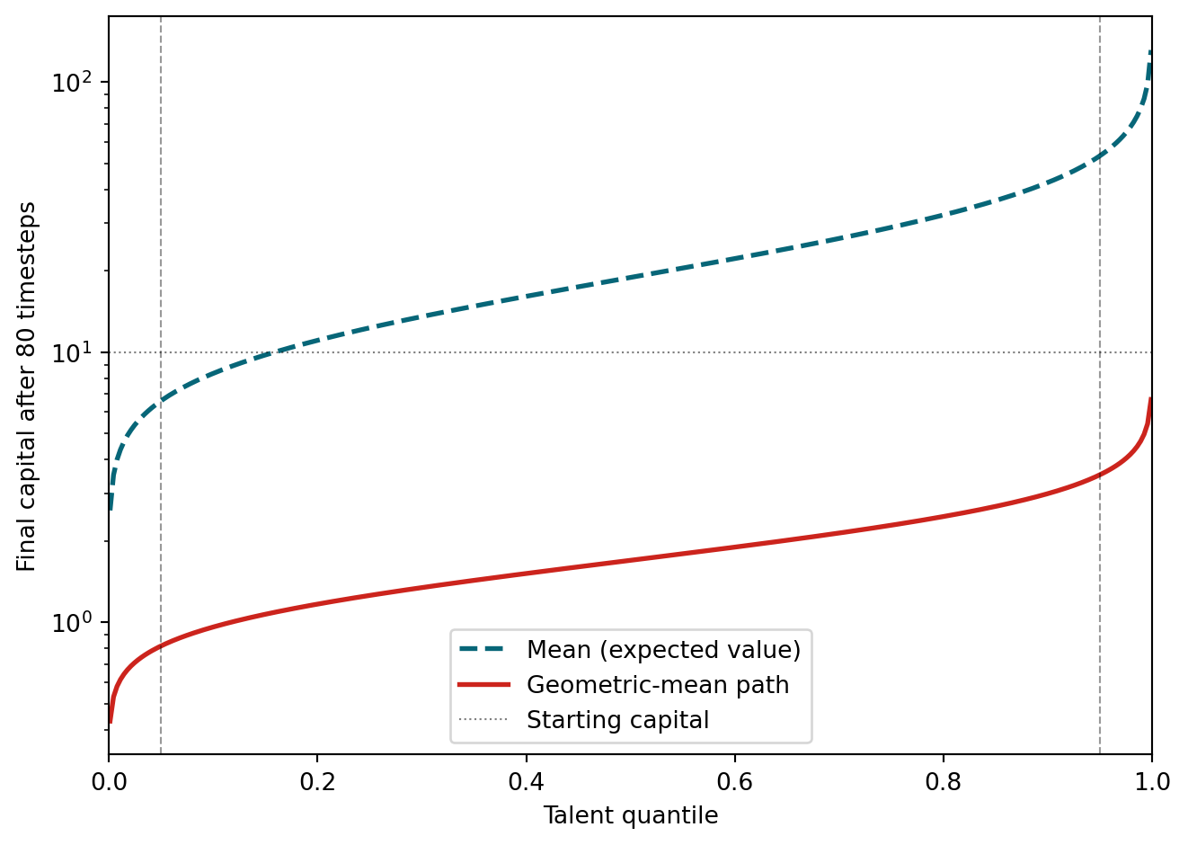
The expected value of each timestep multiplier is \(E[m] = 2 p_\text{double} + 1 \cdot p_\text{same} + 0.5 \cdot p_\text{halve}\), which is above 1 for talent > 0.5. But capital is a multiplicative process — the long-run growth rate is governed by the geometric mean of the per-step multiplier: \(\exp(p_\text{double} \ln 2 + p_\text{halve} \ln 0.5)\). This geometric mean is below 1 for all talent < 1, meaning capital shrinks on a typical path even though the arithmetic mean grows.

def expected_value(quantile, starting_capital=STARTING_CAPITAL, n_timesteps=N_TIMESTEPS):
    p_halve, p_same, p_double = tvl_probabilities(quantile)
    per_step_ev_multiplier = p_double * 2.0 + p_same * 1.0 + p_halve * 0.5
    return starting_capital * per_step_ev_multiplier ** n_timesteps

def geometric_mean_value(quantile, starting_capital=STARTING_CAPITAL, n_timesteps=N_TIMESTEPS):
    """Capital implied by the geometric-mean growth rate (typical-path estimate)."""
    p_halve, p_same, p_double = tvl_probabilities(quantile)
    geo_multiplier = np.exp(p_double * np.log(2) + p_halve * np.log(0.5))
    return starting_capital * geo_multiplier ** n_timesteps

for q, label in [(0.5, "50th"), (0.95, "95th"), (0.999, "99.9th"), (0.99999, "99.999th")]:
    ev = expected_value(q)
    gm = geometric_mean_value(q)
    print(f"{label:10s} percentile → mean: {ev:8.2f}   geo-mean path: {gm:7.4f}  (started at {STARTING_CAPITAL})")

50th       percentile → mean:    18.92   geo-mean path:  1.6958  (started at 10.0)
95th       percentile → mean:    53.39   geo-mean path:  3.5177  (started at 10.0)
99.9th     percentile → mean:   131.42   geo-mean path:  6.6792  (started at 10.0)
99.999th   percentile → mean:   230.50   geo-mean path: 10.0000  (started at 10.0)

The mean and the geometric-mean path tell completely different stories. The mean grows — a 95th-percentile person has an expected final capital over 50. But the geometric-mean path shrinks for every talent level below perfect: a 95th-percentile person’s typical-path capital is about 3.5, down from 10. Only someone with literally perfect talent (\(T = 1\)) has a non-shrinking geometric mean.

This is the signature of a multiplicative process. A few people get lucky runs — several doublings without any halvings — and their enormous gains pull the arithmetic mean far above what most people actually experience. The mean is dominated by rare winners; the geometric mean reflects typical long-run growth.

A caveat: over a finite horizon like 80 steps, variance is high enough that extremely talented individuals still have a meaningful chance of coming out ahead. The geometric mean governs the long-run typical path, but at 80 steps we’re not yet in the long run — the distribution of outcomes is wide, and luck can easily overcome the downward drift for any individual. This doesn’t rescue the model’s claim, though: it just means that which talented people succeed is still driven by luck.

quantiles = np.linspace(0.001, 0.999, 300)

fig, ax = plt.subplots(figsize=(7, 5))
evs = [expected_value(q) for q in quantiles]
gms = [geometric_mean_value(q) for q in quantiles]
ax.plot(quantiles, evs, ls="--", lw=2, color="#076678", label="Mean (expected value)")
ax.plot(quantiles, gms, ls="-", lw=2, color="#cc241d", label="Geometric-mean path")
ax.axhline(STARTING_CAPITAL, color="black", lw=0.8, ls=":", alpha=0.5, label="Starting capital")

for q in (0.05, 0.95):
    ax.axvline(q, color="black", lw=0.8, ls="--", alpha=0.4)

ax.set_xlim(0, 1)
ax.set_xlabel("Talent quantile")
ax.set_ylabel("Final capital after 80 timesteps")
ax.set_yscale("log")
ax.legend()
plt.tight_layout()
plt.show()

Figure 2: Mean (dashed) vs geometric-mean path (solid) after 80 timesteps. The arithmetic mean grows with talent, but the geometric-mean path — reflecting typical long-run growth — stays well below starting capital for all realistic talent levels. Only perfect talent (T = 1) breaks even.

Concluding Thoughts

The TvL paper’s conclusion — that luck dominates talent — is essentially a restatement of its inputs. Two design choices do most of the work:

1. Tiny talent bandwidth. The difference in doubling probability between the 5th and 95th percentile of talent is only ~2.6 percentage points. With such narrow dynamic range, talent can barely move the needle.

2. Asymmetric multipliers. Unlucky events halve your capital regardless of talent, but lucky events only help if you’re talented enough to capitalize. In a multiplicative process, this asymmetry means the typical person loses capital over time even though the average grows — the gains are concentrated in a lucky few.

These are modeling choices, not discoveries about the world. The simulation doesn’t demonstrate that luck dominates talent — it assumes a structure where that outcome is nearly inevitable. This is not to say luck is unimportant in real life; it may well dominate. But this particular model can’t tell us that.

Further Reading

• ArcheoThoughts: “Luck is very important, but just how insignificant is talent?” — another critique identifying the downward pressure on capital in the TvL model.
• Ergodicity Economics by Ole Peters — the formal mathematical framework for why geometric means diverge from arithmetic means in multiplicative processes.
• The Kelly Criterion — the classic solution for maximizing geometric growth under uncertainty.
• The Success Equation by Michael Mauboussin — on how luck becomes dominant when skill levels converge (“the Paradox of Skill”).
• Naval Ravikant on the four kinds of luck — challenges the assumption that luck is purely external by explaining how talent and agency can increase the frequency of lucky events.

Appendix: Estimating p_event

The paper does not state \(p_\text{event}\) directly. We infer it by finding values that reproduce the maximum number of unlucky events seen in the paper’s Figure 5b (approximately 15 events across 1,000 people). The plot below sweeps p_event over 50 simulation trials; our best estimate of 0.16 sits in the center of the plausible range.

p_event_low      = 0.11
p_event_estimate = 0.16
p_event_high     = 0.21

p_events = np.linspace(0.0, 0.5, 250)
trial_rng = np.random.default_rng(seed=42)

fig, ax = plt.subplots(figsize=(7, 4))
for trial in range(50):
    max_unlucky = []
    for pe in p_events:
        n_events = (trial_rng.random((N_PEOPLE, N_TIMESTEPS)) < pe).sum(axis=1)
        n_lucky  = np.array([trial_rng.binomial(n, P_LUCKY) for n in n_events])
        max_unlucky.append((n_events - n_lucky).max())
    ax.plot(p_events, max_unlucky, lw=0.4, color="#076678", alpha=0.5)

ax.axhline(15, color="#cc241d", lw=2, label="Observed max unlucky events (paper Fig. 5b)")
ax.axvline(p_event_low,      color="black", lw=1.5, ls=":",  label="Our estimated range")
ax.axvline(p_event_high,     color="black", lw=1.5, ls=":")
ax.axvline(p_event_estimate, color="black", lw=2.0, ls="--", label="Best estimate (0.16)")
ax.set_xlim(0, 0.5)
ax.set_ylim(0, 40)
ax.set_xlabel("p_event")
ax.set_ylabel("Max unlucky events across 1,000 people")
ax.legend(fontsize=9)
plt.tight_layout()
plt.show()

Figure 3: Maximum unlucky events per person across 50 simulation trials, for different values of p_event. The paper’s Figure 5b shows a maximum of ~15 unlucky events; our estimate of p_event=0.16 sits in the middle of the plausible range.